5 Rcpp or how to easily embed C++ code into a package
Rcpp (“R-C-Plus-Plus”) is a package which facilitates the interface between C++ and . is an interpreted language, a feature that makes a number of things easy (including giving us access to the console in which we can evaluate code and variables on the fly). Nevertheless, this ease of use is counterbalanced by larger computation times compared to lower level languages such as C, Fortran and C++ (but which require compilation).
The curious reader is directed towards the online book Rcpp for everyone by Masaki E. Tsuda, which is a very thorough and complete resource for understanding how to use Rcpp, in complement to the introduction that can be found in the “Rcpp” section of Hadley Wickham’s book Advanced R3.
5.1 First function in Rcpp
👉 Your turn !
To make your package ready for use with
Rcpp, start by running the following command:usethis::use_rcpp()See the changes made
You should also add the following 2 Roxygen comments in the general help page of the package, as indicated in the console:
#' @useDynLib mypkgr
#' @importFrom Rcpp sourceCpp, .registration = TRUE
NULL
We are now going to create a first function in Rcpp to invert a matrix. For this, we will use the C++ library Armadillo. It is a modern and simple linear algebra library, highly optimized, and interfaced with via the RcppArmadillo package.
C++ is not a very different language from . The main differences that will have an impact for us:
C++is very efficient for for loops (including nested for loops – ⚠️ there is often one order that is faster than the other, due to the wayC++allocates and walks through memory).Each command must end with a semicolon
;.C++ is a typed language: you must declare the type of each variable before you can use it in the code.
👉 Your turn !
- Create a new
C++file from RStudio (via theFile>New File>C++ Filemenu), and save it in thesrcfolder. Take the time to read it and try to understand each line.- Compile and load your package (via the “Install and Restart” button) and try using the
timesTwo()function from the console.- Install the
RcppArmadillo👉 package, and don’t forget to make the necessary additions toDESCRIPTION(useusethis::use_rcpp_armadillo())- Using Hadley Wickham’s introduction to
Rcppin his book Advanced R, as well as the documentation for theRcppArmadillopackage and for theC++library Armadillo, try to write a short functioninvC()inC++that computes the inverse of a matrix.- When you have successfully compiled your
invCfunction and it is accessible from , create amvnpdf_invC()function from themvnpdfsmartimplementation replacing only the matrix inverse calculations with a call toinvC.- Evaluate the performance gain of this new implementation
mvnpdf_invC.
n <- 1000
mb <- microbenchmark(mvtnorm::dmvnorm(matrix(1.96, nrow = n, ncol = 2)),
                     mvnpdf(x=matrix(1.96, nrow = 2, ncol = n), Log=FALSE),
                     mvnpdfsmart(x=matrix(1.96, nrow = 2, ncol = n), Log=FALSE),
                     mvnpdfoptim(x=matrix(1.96, nrow = 2, ncol = n), Log=FALSE),
                     mvnpdf_invC(x=matrix(1.96, nrow = 2, ncol = n), Log=FALSE),
                     times=100L)
mb
## Unit: microseconds
##                                                            expr      min
##              mvtnorm::dmvnorm(matrix(1.96, nrow = n, ncol = 2))   26.363
##       mvnpdf(x = matrix(1.96, nrow = 2, ncol = n), Log = FALSE) 1678.868
##  mvnpdfsmart(x = matrix(1.96, nrow = 2, ncol = n), Log = FALSE) 1156.036
##  mvnpdfoptim(x = matrix(1.96, nrow = 2, ncol = n), Log = FALSE)  670.104
##  mvnpdf_invC(x = matrix(1.96, nrow = 2, ncol = n), Log = FALSE) 1146.934
##        lq       mean   median        uq      max neval
##    55.391   68.27074   66.625   82.7175  154.939   100
##  1787.313 1941.00519 1885.242 1989.9145 4067.651   100
##  1221.677 1320.32505 1261.139 1299.5155 3464.090   100
##   712.129  792.31475  727.914  746.3845 3080.002   100
##  1226.023 1362.15079 1269.421 1305.4400 3827.678   100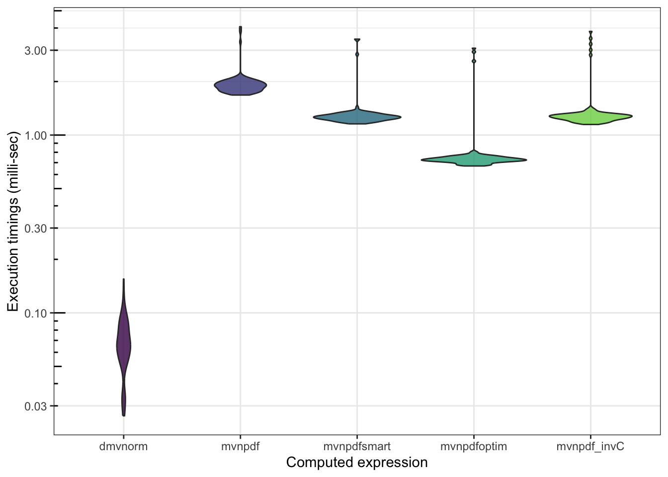
5.2 Optimize thanks to C++
As a general rule, not much computational time is gained by replacing an optimized function with a C++ function. Indeed, most of the base functions are in fact already wrappers around well optimized C or Fortran routines. The gain is then limited to the suppression of argument checking and type management (which is there for a reason!).
👉 Your turn !
From
mvnpdfsmart, propose a complete implementation inC++for computating the density of the multivariate Normal distributionmvnpdfsmartC().Evaluate the performance gain of this new implementation
mvnpdfsmartC.
You can download our proposal for mvnpdfsmartC.cpp here.
For (relatively small) additional speed gain (at the cost of code readability!), you can have a look at our optimized Armadillo C++ implementation in mvnpdfoptimC.cpp.
Finally, we asked LeChat from Mistral AI to propose improvements over this last mvnpdfoptimC() function and it delivered an additional few microseconds speedup implemented in mvnpdfC_LeChat.cpp.
n <- 1000
mb <- microbenchmark(mvtnorm::dmvnorm(matrix(1.96, nrow = n, ncol = 2)),
                     mvnpdf(x=matrix(1.96, nrow = 2, ncol = n), Log=FALSE),
                     mvnpdfsmart(x=matrix(1.96, nrow = 2, ncol = n), Log=FALSE),
                     mvnpdfoptim(x=matrix(1.96, nrow = 2, ncol = n), Log=FALSE),
                     mvnpdf_invC(x=matrix(1.96, nrow = 2, ncol = n), Log=FALSE),
                     mvnpdfsmartC(x=matrix(1.96, nrow = 2, ncol = n), mean = rep(0, 2), varcovM = diag(2), Log=FALSE),
                     mvnpdfoptimC(x=matrix(1.96, nrow = 2, ncol = n), mean = rep(0, 2), varcovM = diag(2), Log=FALSE),
                     mvnpdfC_LeChat(x=matrix(1.96, nrow = 2, ncol = n), mean = rep(0, 2), varcovM = diag(2), Log=FALSE),
                     times=100L)
mb
## Unit: microseconds
## expr
## mvtnorm::dmvnorm(matrix(1.96, nrow = n, ncol = 2))
## mvnpdf(x = matrix(1.96, nrow = 2, ncol = n), Log = FALSE)
## mvnpdfsmart(x = matrix(1.96, nrow = 2, ncol = n), Log = FALSE)
## mvnpdfoptim(x = matrix(1.96, nrow = 2, ncol = n), Log = FALSE)
## mvnpdf_invC(x = matrix(1.96, nrow = 2, ncol = n), Log = FALSE)
## mvnpdfsmartC(x = matrix(1.96, nrow = 2, ncol = n), mean = rep(0, 2), varcovM = diag(2), Log = FALSE)
## mvnpdfoptimC(x = matrix(1.96, nrow = 2, ncol = n), mean = rep(0, 2), varcovM = diag(2), Log = FALSE)
## mvnpdfC_LeChat(x = matrix(1.96, nrow = 2, ncol = n), mean = rep(0, 2), varcovM = diag(2), Log = FALSE)
## min lq mean median uq max neval
## 24.231 53.7305 69.04687 65.6615 81.1390 231.240 100
## 1604.740 1781.5115 1952.24083 1883.4170 1986.0400 4263.508 100
## 1146.606 1221.7385 1323.93387 1273.2345 1313.9885 3622.350 100
## 665.840 706.3685 737.18656 739.8450 755.4045 932.012 100
## 1151.280 1202.4480 1390.74747 1261.7955 1310.7495 3727.720 100
## 33.497 35.6085 38.98321 38.1095 41.0205 76.014 100
## 18.204 20.1925 23.48234 21.4635 23.4725 144.607 100
## 14.596 16.7895 18.60129 17.7735 19.4955 36.572 100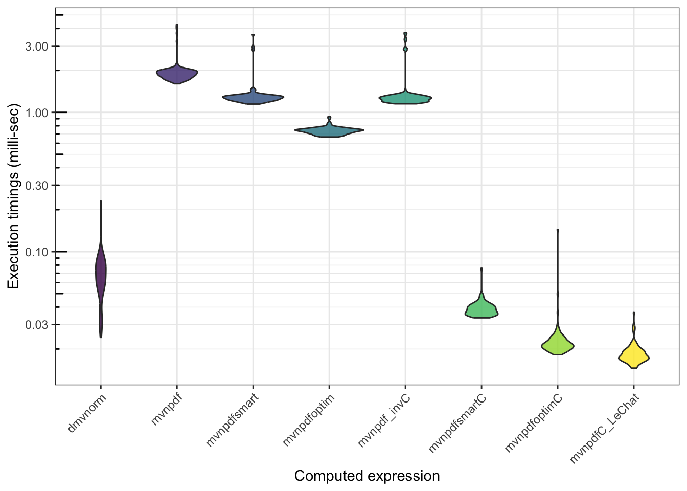
Note that Rcpp functions can be used outside of a package architecture thanks to the Rcpp::sourceCpp() function. But, as we have seen that it is always desirable to manage all of one’s code inside a package, it is unlikely that you will need this !