4 Profiling code
Profiling is about determining which part of the code take the most time to compute (and also memory-wise). Once you have found the block of code that takes the longest time to execute, our goal is only to optimize that small part of the code.
To get a profiling of the code below, select the lines of code of interest and go to the “Profile” menu then “Profile Selected Lines”. It uses the package profvis, and in particular its profvis() function.
n <- 10e4
pdfval <- mvnpdf(x=matrix(1.96, nrow = 2, ncol = n), Log=FALSE)
OK, OK, we get it ! Concatenating a vector as you go in a loop is really not a good idea.
4.1 Comparison with an improved implementtation of mnvpdf().
Consider a new version of mvnpdf(), called mvnpdfsmart(). Download the file, and then include it in the package.
Now profile the following command:
n <- 10e4
pdfval <- mvnpdfsmart(x=matrix(1.96, nrow = 2, ncol = n), Log=FALSE)
We have indeed removed the main computational bottleneck, and we can now learn in a more detailed way what takes time in our function.
To confirm that mvnpdfsmart() is indeed much faster than mvnpdf() we can make a comparison using microbenchmark():
n <- 1000
mb <- microbenchmark(mvnpdf(x = matrix(1.96, nrow = 2, ncol = n), Log = FALSE),
                     mvnpdfsmart(x = matrix(1.96, nrow = 2, ncol = n),
                                 Log = FALSE),
                     times=100L)
mb
## Unit: milliseconds
## expr min
## mvnpdf(x = matrix(1.96, nrow = 2, ncol = n), Log = FALSE) 4.898052
## mvnpdfsmart(x = matrix(1.96, nrow = 2, ncol = n), Log = FALSE) 3.808992
## lq mean median uq max neval cld
## 4.976044 6.081604 5.293864 6.719299 15.590539 100 a
## 3.862859 4.165044 3.925445 4.211289 6.300621 100 b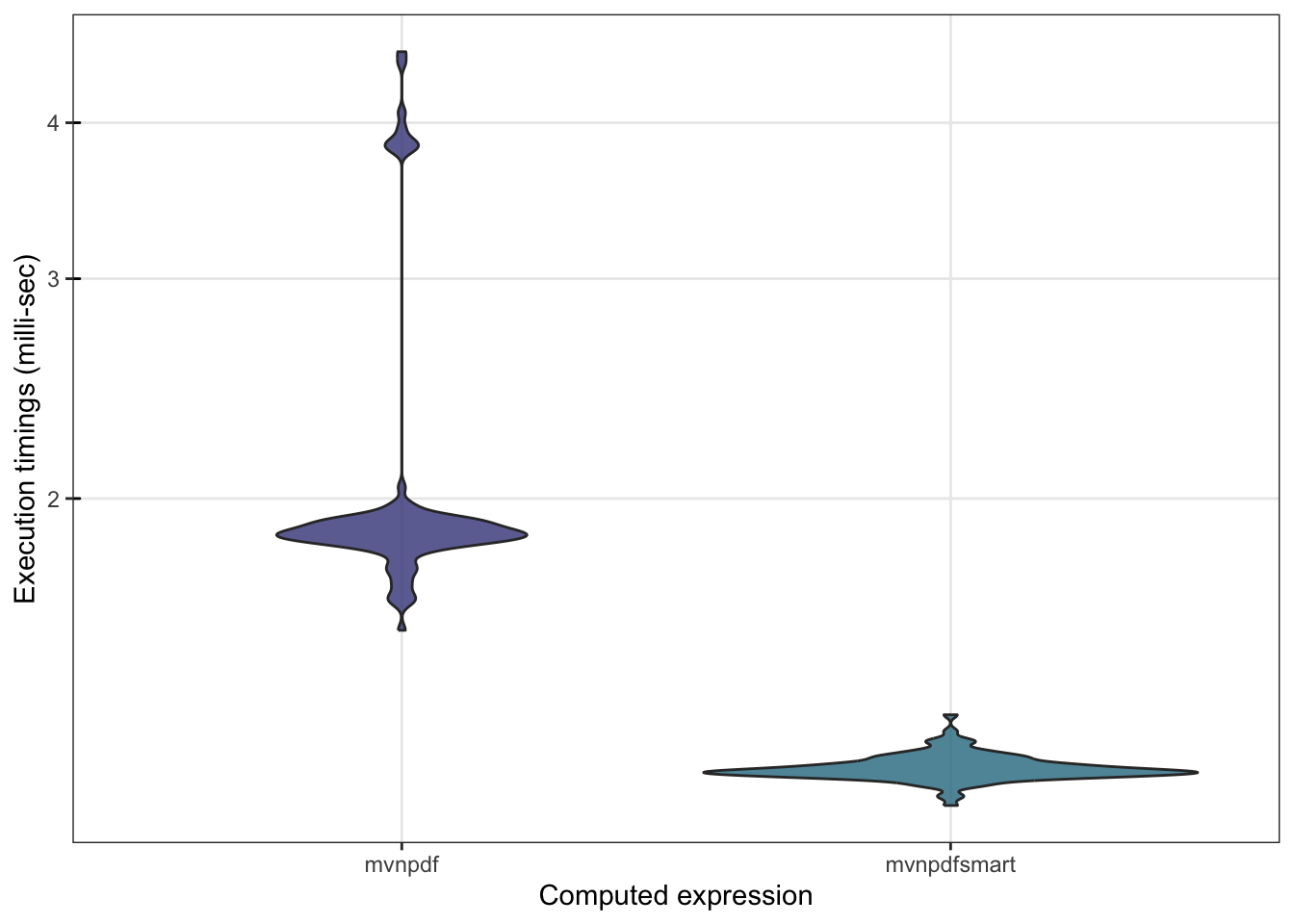
We can also check whether mvnpdfsmart() becomes competitive with dmvnorm():
n <- 1000
mb <- microbenchmark(mvtnorm::dmvnorm(matrix(1.96, nrow = n, ncol = 2)),
                     mvnpdf(x=matrix(1.96, nrow = 2, ncol = n), Log=FALSE),
                     mvnpdfsmart(x=matrix(1.96, nrow = 2, ncol = n), Log=FALSE),
                     times=100L)
mb
## Unit: microseconds
## expr min
## mvtnorm::dmvnorm(matrix(1.96, nrow = n, ncol = 2)) 81.661
## mvnpdf(x = matrix(1.96, nrow = 2, ncol = n), Log = FALSE) 5781.571
## mvnpdfsmart(x = matrix(1.96, nrow = 2, ncol = n), Log = FALSE) 3976.651
## lq mean median uq max neval cld
## 205.3415 492.5964 261.2015 311.195 12650.10 100 a
## 13190.7880 15189.2731 13696.1925 15173.957 41892.14 100 b
## 11062.0900 12206.9655 11317.6515 12046.051 34608.32 100 c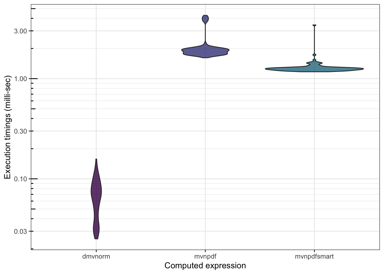
There is still work to be done…
4.2 Comparison with an optimized pure implementation
After several research, tests, trials and errors, Boris arrived at an optimized version using capabilities.
Include this mvnpdfoptim() function in your package, and then profile it:
And the microbenchmark() that goes with it:
n <- 1000
mb <- microbenchmark(mvtnorm::dmvnorm(matrix(1.96, nrow = n, ncol = 2)),
                     mvnpdf(x=matrix(1.96, nrow = 2, ncol = n), Log=FALSE),
                     mvnpdfsmart(x=matrix(1.96, nrow = 2, ncol = n), Log=FALSE),
                     mvnpdfoptim(x=matrix(1.96, nrow = 2, ncol = n), Log=FALSE),
                     times=100L)
mb
## Unit: microseconds
## expr min
## mvtnorm::dmvnorm(matrix(1.96, nrow = n, ncol = 2)) 167.605
## mvnpdf(x = matrix(1.96, nrow = 2, ncol = n), Log = FALSE) 4933.151
## mvnpdfsmart(x = matrix(1.96, nrow = 2, ncol = n), Log = FALSE) 3853.252
## mvnpdfoptim(x = matrix(1.96, nrow = 2, ncol = n), Log = FALSE) 2316.105
## lq mean median uq max neval cld
## 198.0895 395.4377 245.9185 306.656 2941.054 100 a
## 12889.4015 13346.1281 13329.9065 13728.991 27165.915 100 b
## 10818.0335 11112.3187 11159.0380 11284.658 29226.204 100 c
## 6748.6690 6634.5182 6888.6625 6984.056 16913.422 100 d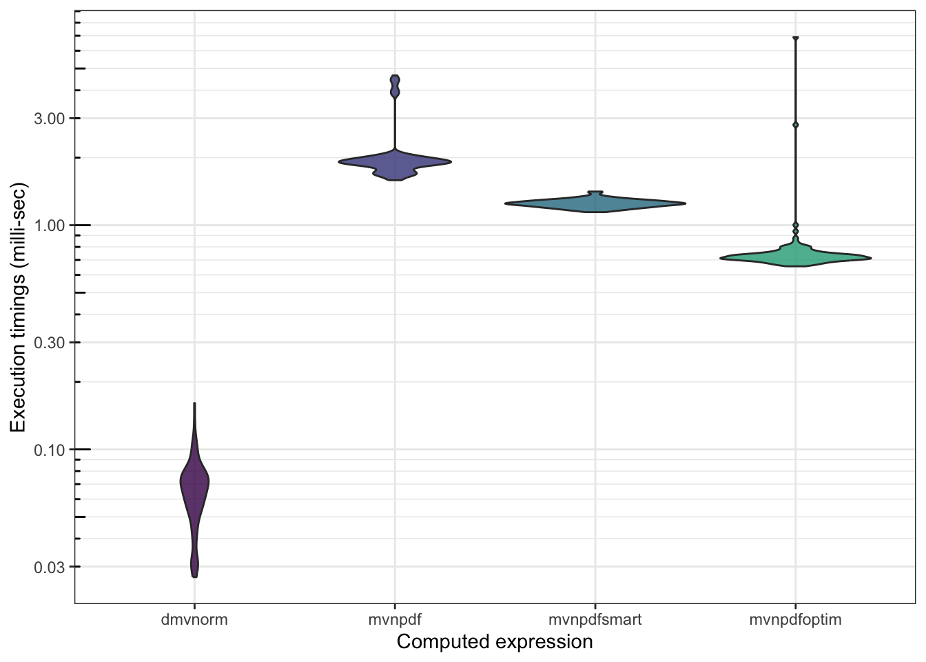
Finally, we can profile the dmvnorm() function:
profvis::profvis(mypkgr::my_dmvnorm(matrix(1.96, nrow = n, ncol = 2)))You can download the my_dmvnorm() function [here](here and include it in your package, in order to have the source code available in the profile result.