3 Measuring and comparing execution times

The first step before optimizing a code is to measure its execution time, in order to compare timings between different implementations.

For this section and the following we refer to the book Advanced R by Hadley Wickham ³, freely available online.

3.1 Measuring execution times with system.time()

To measure the execution time of an command, you can use the native system.time() function like this:

obs <- matrix(rep(1.96, 2), nrow=2, ncol=1)
system.time(mvnpdf(x=obs, Log=FALSE))

##    user  system elapsed 
##   0.001   0.000   0.003

The problem that appears in this example is that the execution is so fast that system.time() displays 0 (or a very close value) that will be impossible to compare to an hopefully faster implementation. Also, we see that there is some variability when we run the command several times.

Thus if we want to compare our code with the mvtnorm::dmvnorm() function, we can’t use system.time():

obs <- rep(1.96, 2)
system.time(mvtnorm::dmvnorm(obs))

##    user  system elapsed 
##   0.003   0.001   0.014

We could imagine that we need to increase the complexity of our calculation to be able to compare them, but there is actually a better way: use the microbenchmark package !

3.2 Compare execution times with microbenchmark()

As its name indicates, this package allows to compare execution times even when they are very fast. Moreover, each benchmarked expression will be repeatedly evaluated a certain number of times, thus stabilizing its timing estimations.

library(microbenchmark)
mb <- microbenchmark(mvtnorm::dmvnorm(rep(1.96, 2)),
                     mvnpdf(x = matrix(rep(1.96,2)), Log = FALSE),
                     times = 1000)

## Warning in microbenchmark(mvtnorm::dmvnorm(rep(1.96, 2)), mvnpdf(x =
## matrix(rep(1.96, : less accurate nanosecond times to avoid potential integer
## overflows

mb

## Unit: microseconds
##                                           expr    min     lq     mean median
##                 mvtnorm::dmvnorm(rep(1.96, 2)) 20.049 20.992 24.07823 21.566
##  mvnpdf(x = matrix(rep(1.96, 2)), Log = FALSE) 18.122 19.188 20.55752 19.639
##      uq      max neval cld
##  23.247 1598.508  1000  a 
##  20.992  103.115  1000   b

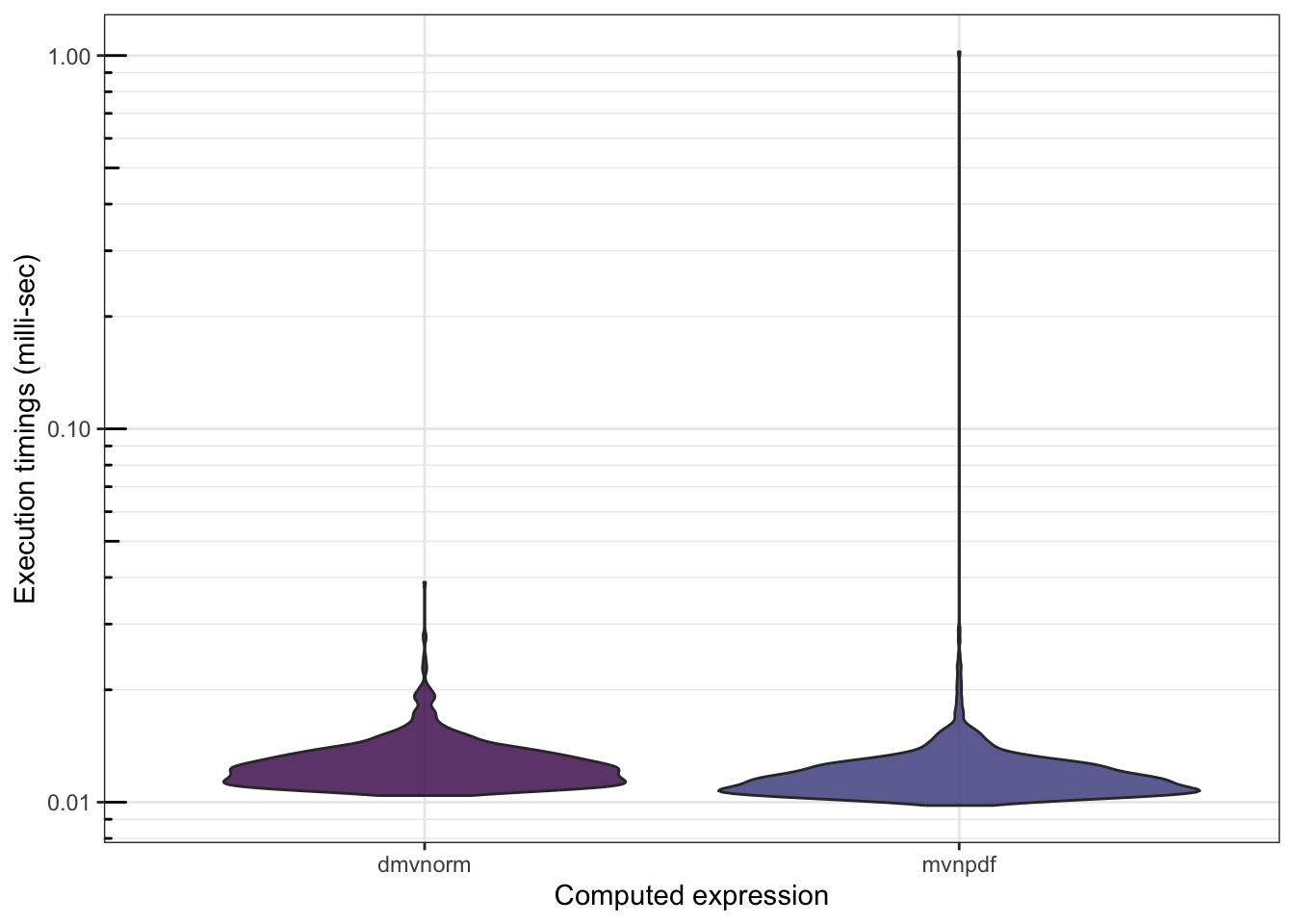
Both mvnpdf() and dmnvorm() functions being able to take a matrix as input, we can also compare their speeds in this setting:

n <- 100
mb <- microbenchmark(mvtnorm::dmvnorm(matrix(1.96, nrow = n, ncol = 2)),
                     mvnpdf(x=matrix(1.96, nrow = 2, ncol = n), 
                            Log=FALSE),
                     times=100)
mb

## Unit: microseconds
##                                                       expr     min      lq
##         mvtnorm::dmvnorm(matrix(1.96, nrow = n, ncol = 2))  23.206  24.518
##  mvnpdf(x = matrix(1.96, nrow = 2, ncol = n), Log = FALSE) 266.746 271.338
##      mean   median      uq     max neval cld
##   27.9333  25.7275  27.265  79.458   100  a 
##  279.4019 274.3720 281.629 331.198   100   b

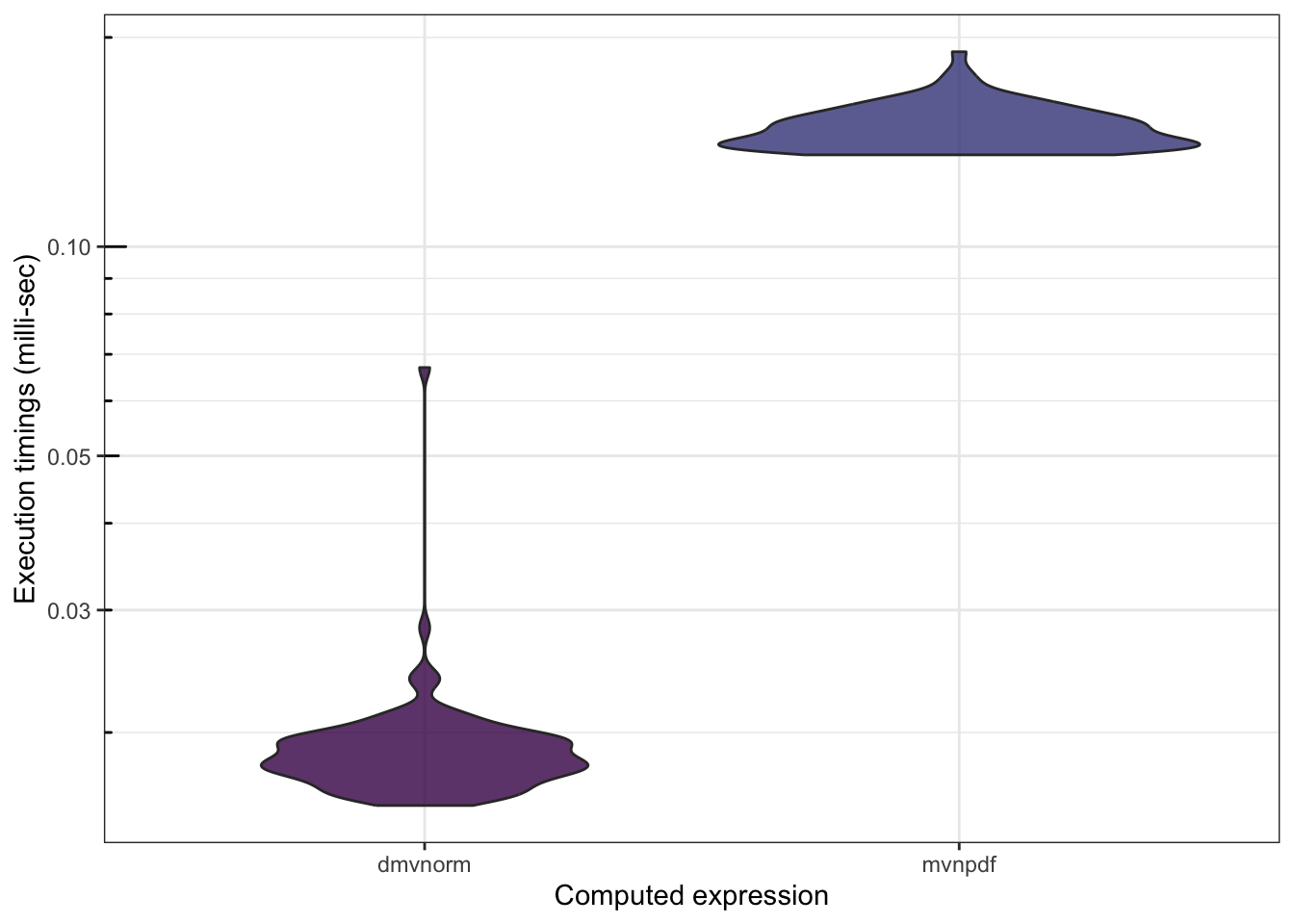
Something happened… And we will find out what exactly is causing this issue in what comes next.