6 R code Parallelization
6.1 Introduction to parallel execution in
Apart from optimizing the code and the algorithms, another way to get a high performing code is to take advantage of the parallel architectures of modern computers. The goal is then to parallelize a code in order to perform simultaneous operations on distinct parts of the same problem, using different computing cores. This does not reduce the total computation time needed, but the set of operations is executed faster, resulting in an overall user speed-up.
There is a significant number of algorithms that are so-called “embarrassingly parallel”, i.e. whose computations can be broken down into several independent sub-computations. In statistics, it is often easy and straightforward to parallelize according to different observations or different dimensions. Typically, these are operations that can be written in the form of a loop whose operations are independent from one iteration to the next.
The necessary operations to execute code in parallel are as follows:
Start \(m\) “worker” processes (i.e. computing cores) and initialize them
Send the necessary functions and data for each task to the workers
Split the tasks into \(m\) operations of similar size and send them to the workers
Wait for all workers to finish their calculations
Collect the results from the different workers
Stop the worker processes
Depending on the platform, several communication protocols are available between cores. Under UNIX systems, the Fork protocol is the most used (it has the benefit of sharing memory), but it is not available under Windows where the PSOCK protocol is used instead (with duplicated memory). Finally, for distributed computing architecture where the cores are not necessarily on the same physical processor, the MPI protocol is generally used. The advantage of the future and future.apply package is that the same code can be executed whatever the hardware configuration.
In the parallel package allows to start and stop a cluster of several worker processes (step 1 and 6). In addition to the parallel package, we will use the future package which allows to manage the worker processes and the communication and articulation with the future.apply package, which in turn allows to manage the dialogue with the workers (sending, receiving and collecting the results – steps 2, 3, 4 and 5).
NB: The free plan on Posit Cloud only includes 1 core.
6.2 First parallel function
👉 Your turn!
Start by writing a simple function that computes the logarithm of \(n\) numbers:
Determine how many cores are available on your computer with the function
future::availableCores()(under Linux, preferparallel::detectCores(logical=FALSE)to avoid overthreading).Load the
futurepackage and using the functionfuture::plan(multisession(workers = XX)), declare a “plan” of parallel computations on your computer (take care to always leave at least one core available to handle other processes).Using one of the *apply functions
future.apply::future_*apply(), compute the log of \(n\) numbers in parallel and concatenate the results into a vector.Compare the execution time with that of a sequential function on the first 100 integers, using the command :
microbenchmark(log_par(1:100), log_seq(1:100), times=10)
library(microbenchmark)
library(future.apply)

log_seq <- function(x) {
  # try this yourself (spoiler alert: it is quite long...):
  # res <- numeric(length(x))
  # for(i in 1:length(x)){
  #   res[i] <- log(x[i])
  # }
  # return(res)
  return(log(x))
}

log_par <- function(x) {
  res <- future_sapply(1:length(x), FUN = function(i) {
    log(x[i])
  })
  return(res)
}

plan(multisession(workers = 3))
mb <- microbenchmark(log_par(1:100), log_seq(1:100), times = 50)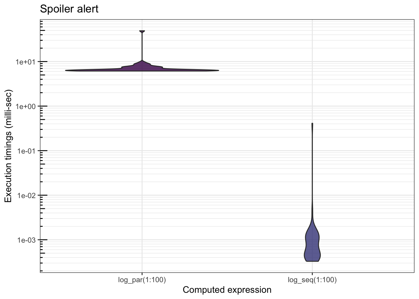
The parallel version runs much slower… Indeed, since the individual tasks are too fast, will spend more time communicating with the cores than doing the actual computations. Hence:
A loop iteration must be relatively long for parallel computing to provide a significant gain in computation time!
By increasing \(n\), we observe a reduction in the difference between the 2 implementations (the parallel computation time increases very slowly compared to the increase of the sequential function).
6.3 Efficient parallelization
We will now look at another use case. Let’s say we have a large array of data with 10 observations for 100,000 variables (e.g. genetic measurements), and we want to compute the median for each of these variables.
## [1] 10 100000For an experienced user, such an operation is easily implemented using apply():
colmedian_apply <- function(x){
  return(apply(X = x, MARGIN = 2, FUN = median))
}
system.time(colmedian_apply(x))
## user system elapsed
## 0.920 0.008 0.929In reality, a (good) for loop is no slower – provided it is nicely programmed:
colmedian_for <- function(x){
  p <- ncol(x)
  ans <- numeric(p)
  for (i in 1:p) {
    ans[i] <- median(x[, i])
  }
  return(ans)
}
system.time(colmedian_for(x))
## user system elapsed
## 0.836 0.007 0.844👉 Your turn! Try to further improve this computation time by parallelizing your code for each of the 100,000 variables. Is there a gain in computation time?
colmedian_par <- function(x){
  res <- future_sapply(1:ncol(x), FUN = function(i) {
          median(x[, i])
    })
  return(res)
}
plan(multisession(workers = 3))
system.time(colmedian_par(x))
## user system elapsed
## 0.089 0.019 0.479
mb <- microbenchmark(colmedian_apply(x),
                     colmedian_for(x),
                     colmedian_par(x),
                     times = 10)
mb
## Unit: milliseconds
## expr min lq mean median uq max neval
## colmedian_apply(x) 861.3462 865.0756 887.7010 886.6892 897.6432 952.0836 10
## colmedian_for(x) 813.4748 834.7167 862.7321 857.8160 892.5319 937.5436 10
## colmedian_par(x) 442.6223 465.5680 469.0186 470.2647 474.9341 493.1818 10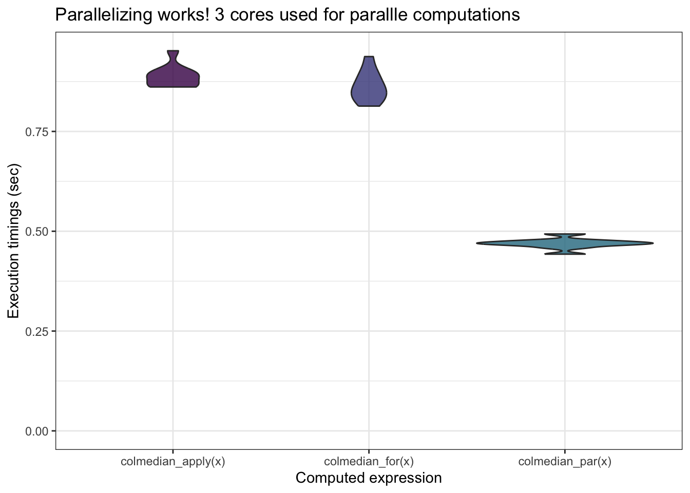
6.3.1 Other “plans” for parallel computations
To run your code (exactly the same code, this is one of the advantages of the future* family packages), you need to set up a “plan” of computations:
On a computer (or a single computer server) under Unix ( Linux, MacOS), you can use
plan(multicore(workers = XX))which is often more efficient. Themultisessionplan always works.On an HPC cluster (like CURTA in Bordeaux), we refer to the package
future.batchtools
6.4 Parallelization in our common theme example
👉 Your turn!
From the function
mvnpdfoptim()and/ormvnpdfsmart(), propose an implementation parallelizing the computations on the observations (columns of \(x\))Compare the execution times for 10 000 observations
plan(multisession(workers = 3))
n <- 10000
mb <- microbenchmark::microbenchmark(
  mypkgr::mvnpdfsmart(x=matrix(1.96, nrow = 2, ncol = n), Log=FALSE),
  mypkgr::mvnpdfsmart_par(x=matrix(1.96, nrow = 2, ncol = n), Log=FALSE),
  times=20)
mb
## Unit: milliseconds
## expr
## mypkgr::mvnpdfsmart(x = matrix(1.96, nrow = 2, ncol = n), Log = FALSE)
## mypkgr::mvnpdfsmart_par(x = matrix(1.96, nrow = 2, ncol = n), Log = FALSE)
## min lq mean median uq max neval
## 12.89093 13.42740 13.9988 13.89615 14.60955 15.24372 20
## 30.37444 31.18175 36.8028 32.78354 33.59276 74.69236 20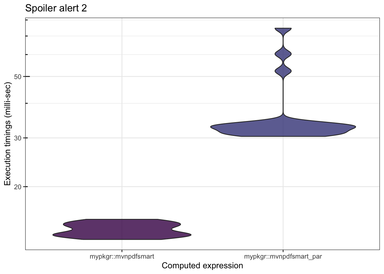
You can download our proposed implementation for mvnpdfsmart_par here.
In this example, the computation time of one iteration is really too fast for the parallel version to be efficient. We artificially add some time on each iteration to illustrate the gain of parallel computing for this example.
plan(multisession(workers = 3))
n <- 10000
system.time(mypkgr::mvnpdfsmart_sleepy(x=matrix(1.96, nrow = 2, ncol = n), Log=FALSE))
## user system elapsed
## 0.210 0.089 12.809
system.time(mypkgr::mvnpdfsmart_sleepy_par(x=matrix(1.96, nrow = 2, ncol = n), Log=FALSE))## user system elapsed
## 0.299 0.013 4.342You can finally clone (or download or fork) our GitHub repository to get all the different implementations directly.
6.5 Conclusion
Parallel computation saves time, but first you have to optimize your code. When parallelizing a code, the gain on the execution time depends above all on the ratio between the communication time and the effective computation time for each task.
Annexe 6.1: Progress bar
The pbapply package allows to get a nice progress bar for parallelized *apply functions execution, and its parallelization capabilities are relatively straightforward to use (very straightforward on both Linux, MacOS, slightly more involved on Windows). Try it out !