4 Profiling the code
Profiling is about determining which part of the code takes the most time to compute (and also memory-wise). Once we have found the block of code that takes the longest time to execute, our goal is only to optimize that small part of the code.
To get a profiling of the code below, select the lines of code of interest and go to the “Profile” menu then “Profile Selected Lines”.
n <- 10e4
pdfval <- mvnpdf(x=matrix(1.96, nrow = 2, ncol = n), Log=FALSE)
It uses the profvis() function of the package profvis, so you can alternatively use it:
OK, OK, we get it! Concatenating a vector as you go in a loop is really not a good idea in .
4.1 Comparison with an improved implementation of mnvpdf().
Consider a new version of mvnpdf(), called mvnpdfsmart(). Download the file, and then include it in the package (i.e., save it into the R/ folder and add minimally the @export Roxygen tag at the top of it, and then document/build your package).
Now profile the following command:
n <- 10e4
pdfval <- mvnpdfsmart(x=matrix(1.96, nrow = 2, ncol = n), Log=FALSE)
We have indeed removed the main computational bottleneck, and we can now learn in a more detailed way what takes time in our function.
To confirm that mvnpdfsmart() is indeed much faster than mvnpdf() we can make a comparison using microbenchmark():
n <- 1000
mb <- microbenchmark(mvnpdf(x = matrix(1.96, nrow = 2, ncol = n), Log = FALSE),
                     mvnpdfsmart(x = matrix(1.96, nrow = 2, ncol = n),
                                 Log = FALSE),
                     times=100L)
mb
## Unit: milliseconds
## expr min
## mvnpdf(x = matrix(1.96, nrow = 2, ncol = n), Log = FALSE) 1.568455
## mvnpdfsmart(x = matrix(1.96, nrow = 2, ncol = n), Log = FALSE) 1.135372
## lq mean median uq max neval
## 1.845020 2.073026 1.874438 1.919477 4.559651 100
## 1.200767 1.216624 1.210914 1.227028 1.342176 100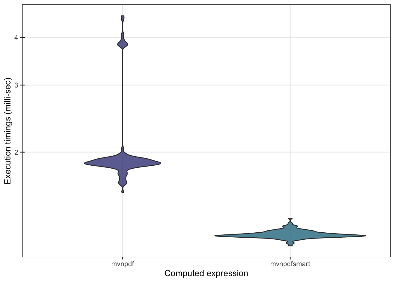
We can also check whether mvnpdfsmart() becomes competitive with dmvnorm():
n <- 1000
mb <- microbenchmark(mvtnorm::dmvnorm(matrix(1.96, nrow = n, ncol = 2)),
                     mvnpdf(x=matrix(1.96, nrow = 2, ncol = n), Log=FALSE),
                     mvnpdfsmart(x=matrix(1.96, nrow = 2, ncol = n), Log=FALSE),
                     times=100L)
mb
## Unit: microseconds
## expr min
## mvtnorm::dmvnorm(matrix(1.96, nrow = n, ncol = 2)) 25.174
## mvnpdf(x = matrix(1.96, nrow = 2, ncol = n), Log = FALSE) 1615.441
## mvnpdfsmart(x = matrix(1.96, nrow = 2, ncol = n), Log = FALSE) 1170.550
## lq mean median uq max neval
## 40.9795 67.13791 69.3105 85.7925 157.809 100
## 1773.1680 2062.47835 1889.2390 1987.5365 4283.188 100
## 1221.0210 1292.04202 1255.2970 1288.5685 3435.841 100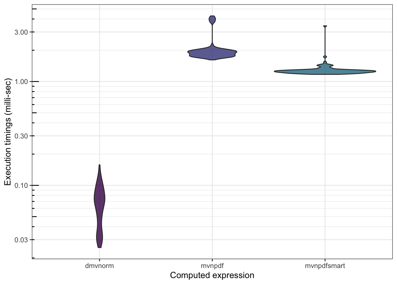
There is still work to be done…
4.2 Comparison with an optimized pure implementation
After several research, tests, trials and errors, Boris arrived at an optimized version using capabilities.
Include this mvnpdfoptim() function in your package, and then profile it:
And the microbenchmark() that goes with it:
n <- 1000
mb <- microbenchmark(mvtnorm::dmvnorm(matrix(1.96, nrow = n, ncol = 2)),
                     mvnpdf(x=matrix(1.96, nrow = 2, ncol = n), Log=FALSE),
                     mvnpdfsmart(x=matrix(1.96, nrow = 2, ncol = n), Log=FALSE),
                     mvnpdfoptim(x=matrix(1.96, nrow = 2, ncol = n), Log=FALSE),
                     times=100L)
mb
## Unit: microseconds
## expr min
## mvtnorm::dmvnorm(matrix(1.96, nrow = n, ncol = 2)) 26.937
## mvnpdf(x = matrix(1.96, nrow = 2, ncol = n), Log = FALSE) 1587.192
## mvnpdfsmart(x = matrix(1.96, nrow = 2, ncol = n), Log = FALSE) 1143.326
## mvnpdfoptim(x = matrix(1.96, nrow = 2, ncol = n), Log = FALSE) 655.549
## lq mean median uq max neval
## 53.6280 66.21254 66.4610 76.8340 160.802 100
## 1809.1250 2080.14812 1903.7120 1984.8100 4656.493 100
## 1214.0305 1250.16503 1246.5845 1282.2135 1412.696 100
## 703.9495 814.28214 722.4815 746.7945 6903.293 100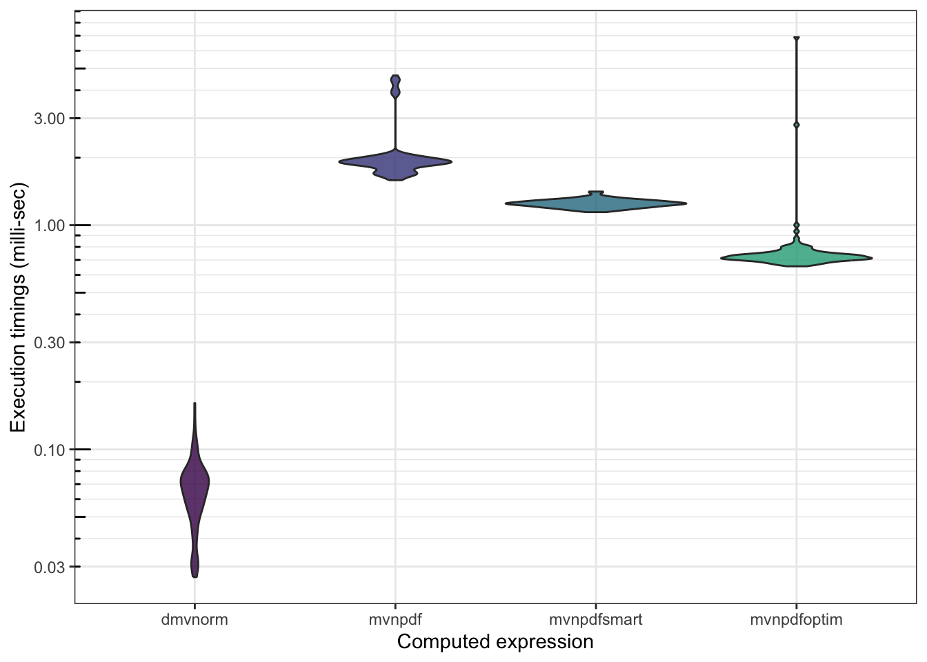
Finally, we can profile the dmvnorm() function:
profvis::profvis(mypkgr::my_dmvnorm(matrix(1.96, nrow = n, ncol = 2)))You can download the my_dmvnorm() function here and include it in your package, in order to have the source code available in the profiling result.